Bollinger Bands are financial charting tools that were developed in the 1980s by John Bollinger. These indicators help investors visualize when stocks break out of a trading range and identify buying and selling opportunities.

There are good reasons to expect Bollinger Bands to work… at least in theory. Researchers have long known that rising stocks tend to keep going up over time. Bollinger Bands uses this “winners keep winning” observation to help investors profit. We also know that investor greed often creates self-fulfilling feedback loops, compounding the momentum effects in illiquid assets. Studies have found that Bollinger Band strategies perform well in less efficient markets dominated by private investors.

But in practice, it’s unclear whether these simple rules work for the average American investor. Western stock markets are relatively efficient and high-frequency trading algorithms dominate many trading platforms. Could a strategy as straightforward as Bollinger Bands still help investors outperform?

How Do Bollinger Bands Work?

Let’s quickly examine how Bollinger Bands work.

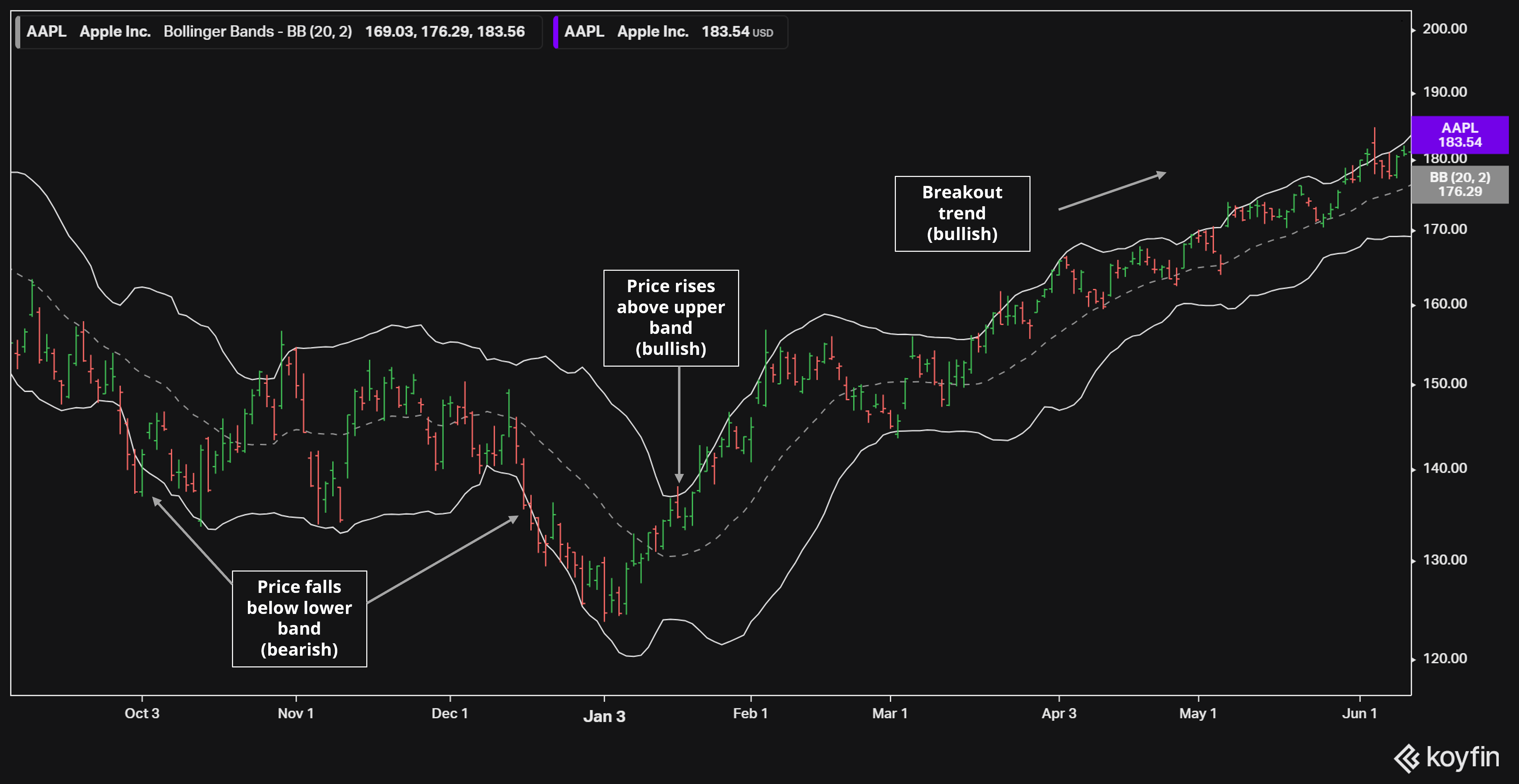
1. Moving Average. First, technical analysts will calculate a moving average of stock prices, typically a 20-day window.
2. Standard Deviation. Next, the volatility of the stock is converted into a standard deviation. This number grows during periods of high volatility and shrinks when prices are more stable.
3. Calculate Upper and Lower Bands. Then, the standard deviation is added to the moving average to determine the upper Bollinger Band and subtracted from the moving average to find the lower band.
4. Trading Strategy. Finally, traders will determine the right strategy using these bands and the ranges they create. The system is often combined with other technical and fundamental indicators.

Momentum-Seeking Strategy

The most common way to use Bollinger Bands is to buy stocks when prices rise above their top band and sell them when they fall below. This is called a “momentum-seeking” strategy and works well for companies that “break out” of trading ranges. Here’s Nvidia (NASDAQ:NVDA) in 2023, where prices jumped from $150 to over $450.

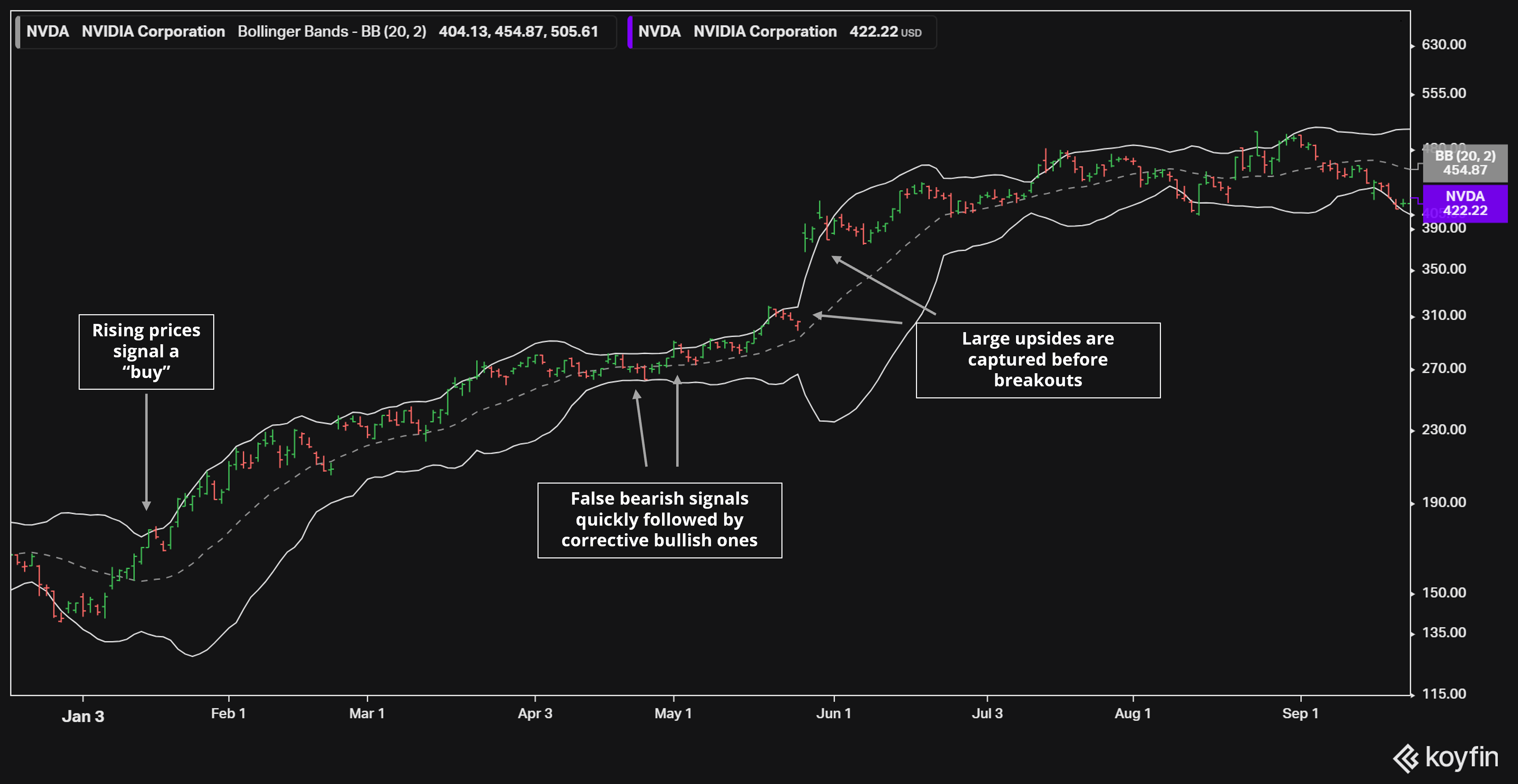
It’s a useful tactic for identifying high-potential stocks early and keeping traders invested as prices rise.

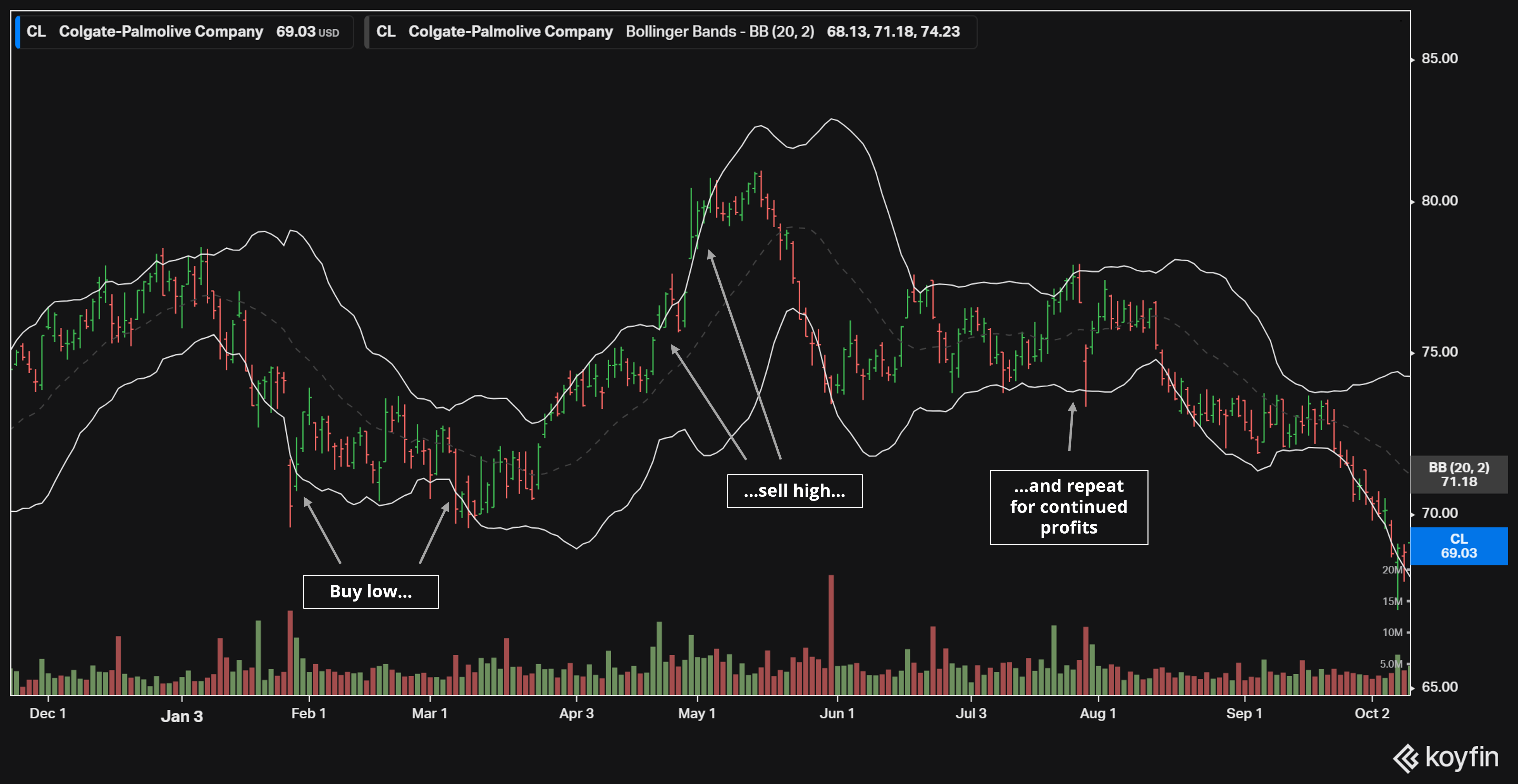
However, the same momentum-seeking Bollinger Band strategy will fail if companies trade in a narrow band. That’s because “buy” signals will trigger toward the top of the markets and “sell” signals happen at the bottom. In other words, investors will be buying high and selling low — a recipe for losses.

Contrarian (Momentum-Avoiding) Strategy

To address this issue, some traders will use Bollinger Bands as a contrarian indicator instead. These investors will use the upper band as an “overbought” signal and the lower band as an “oversold” one. This is particularly useful for companies that trade in a narrow range. Colgate Palmolive (NYSE:CL) (pictured below) is an excellent example of a firm where upswings are followed by reversals — and where contrarian strategies work well.

Advanced Strategies

More complex Bollinger Band strategies also exist. Here are several examples:

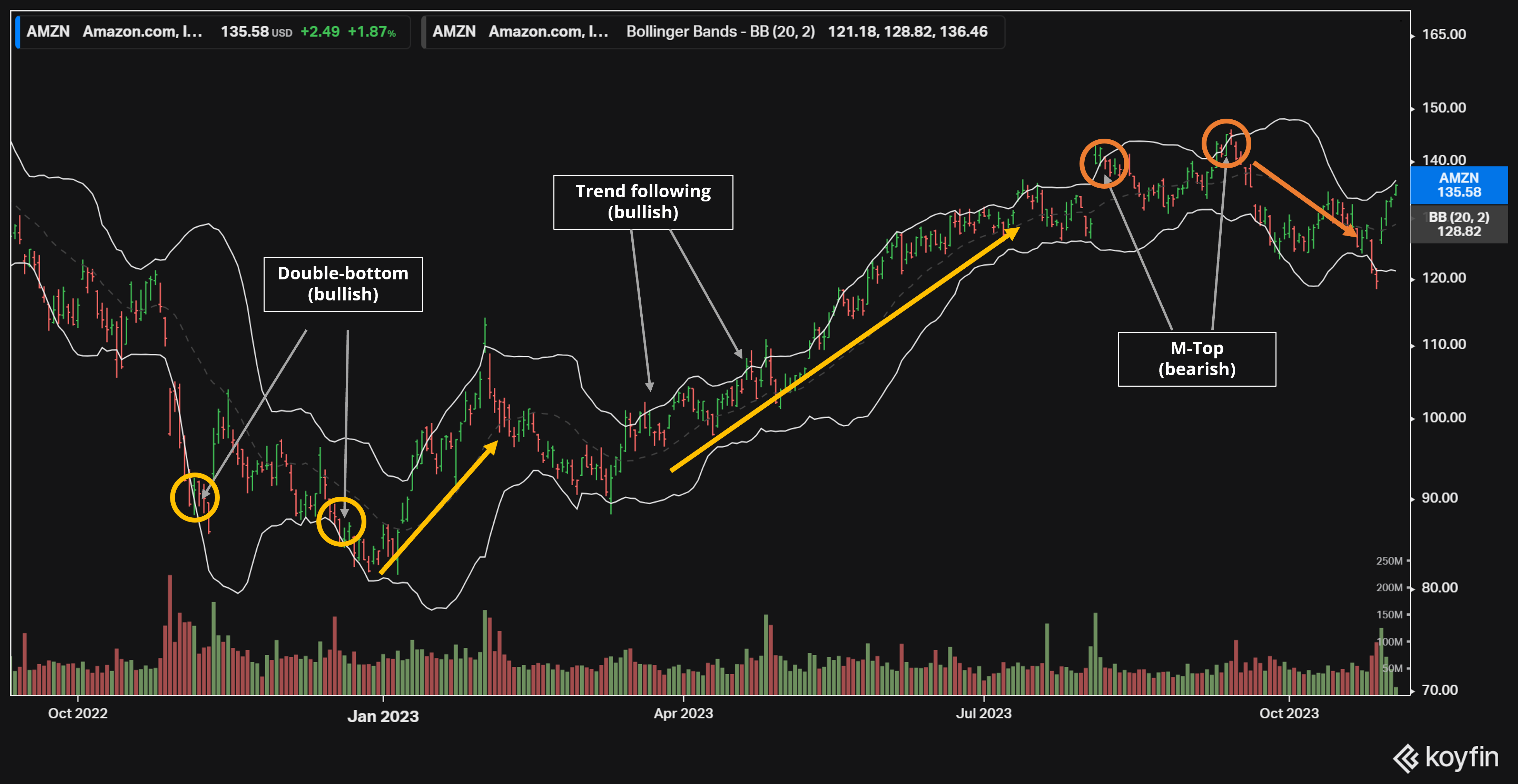
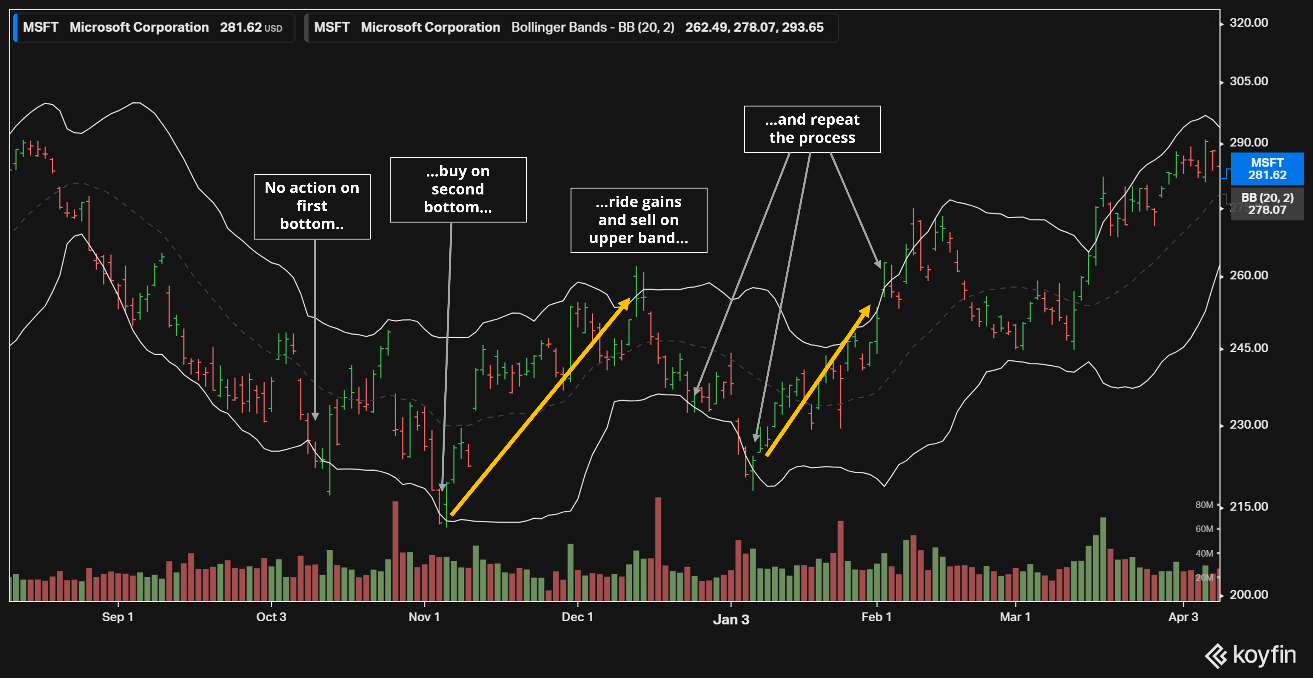
• Double bottom. A “W” shape is formed when falling stocks hit the bottom Bollinger band for the second time. This is often seen as a bullish signal, particularly in commodity markets, since it suggests a large amount of buying demand at the bottom-band level. This can also suggest a concentration of “good-til-canceled” orders in that range.
• M Top. The opposite is often true when stocks hit the top Bollinger band for the second time, creating an inverted “W”… which looks like the letter “M.” This indicates selling pressure at the higher Bollinger Band and often indicates a drawdown can happen from there.
• Trend Following. Finally, chartists will often point to a stock price that “hugs” the upper band. This is a bullish sign, since rising prices will increase the moving average price, which consequently moves the upper Bollinger Band higher.

Do Bollinger Bands Actually Work?

I’ll admit to being a technical analysis skeptic. We know plenty of investors who have become wealthy from fundamental investing. But who has ever heard of anyone becoming a billionaire by drawing lines over stock charts?

However, findings from MarketMasterAI have since changed my mind… at least a little. According to the machine-learning algorithm I developed, share prices strongly predict future returns, especially when paired with analyst estimates, financial data and fundamental analysis. Successful companies that can generate strong returns keep going up, while weak ones take time to melt away. Investors using a quant-based strategy can expect to outperform the market by a 2-to-1 margin over long periods. Technical analysis only gets a bad name because users expect 10X returns from a single metric!

So, how do Bollinger Bands hold up against other momentum-seeking strategies? To test this, I gathered daily pricing data from Refinitiv/Datastream for all Russell 3000 stocks from 2018 to 2023, a five-year window. The index is not rebalanced since we want to capture how the strategy performs when faced with companies that go defunct. After all, the survival rate for all stocks eventually goes to zero over long enough periods and we need to make sure any strategy can deal with failing firms.

For this study, I’ll use a Jupyter Notebook and some essential add-ins like Pandas and Python’s TA library.

Here’s what our database looks like. It’s a straightforward table of dates, stocks and prices for our period.

1. Baseline: Calculate Buy-and-Hold Performance for Benchmarking

First, let’s see what a baseline looks like if an investor bought all Russell 3000 stocks in equal portions on the first trading day of 2018. We’ll assume buyers achieved the close price for the following day to prevent any look-forward bias. Here’s a code snippet to give you an idea of the process. Daily price changes are converted into logarithmic (log) returns and null values are dropped. Here, I’m iterating across all tickers (instead of doing all at once) because the looping method will prove handy later for running different strategies.

# Create empty dataframes to hold results
df_baseline_log_returns = pd.DataFrame(data=df_input["Date"])
                                       
# Create for loop to iterate across all tickers          
df_columns = list(df_input)
for ticker in df_columns[1:]:
    
    df = pd.DataFrame(data=None)
    df["date"] = df_input["Date"]
    df["price"] = df_input[ticker]
    
    # Calculate daily returns and drop nas. Use T+1 prices to prevent lookback bias
    df["next_day_price"] = df["price"].shift(periods=-1)
    df["log_return"] = np.log(df["next_day_price"] / df["price"])
    df.dropna(axis=0, inplace=True)

    # Calculate daily log returns
    df_baseline_log_returns = pd.concat((df_baseline_log_returns,df["log_return"].rename(ticker)),axis=1)

    # Remove dates prior to 2018
    df_baseline_log_returns = df_baseline_log_returns[63:]

Logarithmic returns are especially useful because they conveniently add to the logarithm of the total returns. This shortcut helps us calculate performance numbers in essentially one line of code (bolded). Here’s how it looks in Python code:

df = df_baseline_log_returns[63:] # remove data prior to 2018
date = df["Date"]
log_ret = df.iloc[:, 1:].mean(axis=1)
df_baseline_returns = pd.DataFrame(data={"date": date, "log_return":log_ret})
df_baseline_returns["baseline_returns"] = np.exp(df_baseline_returns["log_return"].cumsum().astype(float))

Some basic graphing then gives us our baseline performance of all Russell 3000 stocks since 2018:

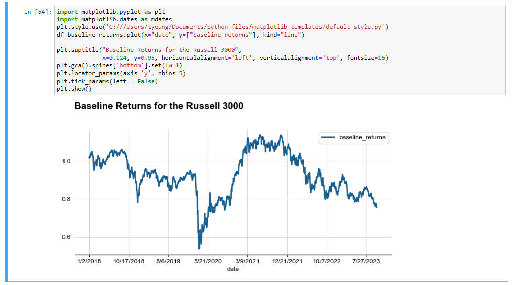
As a quick note, the equal-weighted returns of Russell companies will naturally underperform the actual index since our sample continues to track firms that drop out. We do this to ensure the Russell rebalances don’t “help” our Bollinger Band strategy by cutting out weak players. (The strategy must remove these duds for itself).

2. Momentum-Seeking Bollinger Band Strategies

Next, we look at the most straightforward Bollinger Band strategy:

Buy stocks when they rise above their upper band and sell them short once they hit the lower band.

Here’s a snippet of how that’s calculated using Python’s TA (technical analysis) library:

    # Add Bollinger Band high indicator: registers as +1 when triggered
    df['bb_bbhi'] = indicator_bb.bollinger_hband_indicator()

    # Add Bollinger Band low indicator: registers as +1 when triggered
    df['bb_bbli'] = indicator_bb.bollinger_lband_indicator()

    # Add position: +1 when high triggers, -1 when low triggers. Then forward fill results
    df["position"] = (df.bb_bbhi - df.bb_bbli).astype(float)
    df["position"].replace(0, method='ffill', inplace=True)

This compressed bit of code does the job. After inserting this into our for-loop above and rerunning the summations, we get the following output:

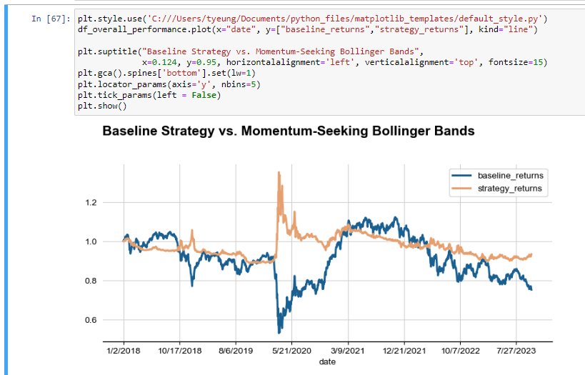
We get some outperformance! Rather than lose 24.8% over the period, we only went down by 6.8%. This was driven by a massive spike during the Covid-19 bear market (when the strategy suddenly shorted all stocks) and holding onto those gains during the 2021 to 2023 drawdown. That tells us that the Bollinger Band strategy might be onto something.

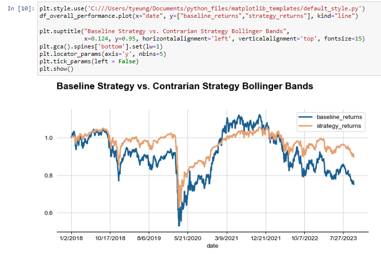
However, many investors understandably can’t short stocks… or at least aren’t willing to endure the stress of a margin call. Let’s re-run the test and turn all short positions into neutral ones. So if a company drops below its lower Bollinger Band, we sell out our position and hold cash. (We’ll assume cash yields zero, but it’s easy enough to change that).

The new code is bolded below and goes back into our for-loop.

    # Add position: +1 when high triggers, -1 when low triggers. Then fowrard fill results
    df["position"] = (df.bb_bbhi - df.bb_bbli).astype(float)
    df["position"].replace(0, method='ffill', inplace=True)
 
    # Then replace all "-1" positions with "0" to signify moving into cash
    df["position"].replace(-1, 0, inplace=True)

Re-running our code still shows Bollinger Bands outperforming! The strategy was quick to sell out of drawdowns in 2018 and 2020. It then captured some of the gains during the recovery, even if it didn’t pick them all.

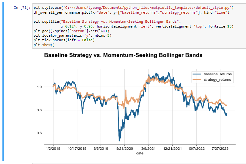
Our momentum-seeking strategy saved us 8.6% underperformance over five years, or roughly an annualized 1.6% return.

(As a side note, we would run all these findings through validation processes before using them in real-life trading. It’s not enough to outperform the market in backtests — you also need to know the probability of false positives and whether the same strategy will work in the future. That’s a little beyond the scope of this study, but please feel free to reach out to our editors if you want to learn more).

3. Contrarian Bollinger Band Strategies

Next, let’s consider the contrarian model. Here, stocks are sold when they rise above their upper Bollinger Band and bought when they fall below. (See the Colgate-Palmolive chart in the intro for a graph of that strategy). This is done by adding a new line of code that simply turns our positions upside down. Positive positions are turned negative and vice versa.

    df["position"] = (df.bb_bbhi - df.bb_bbli).astype(float)
    df["position"].replace(0, method='ffill', inplace=True)
    df["position"] = -df["position"]

Here are the results if shorting is allowed…

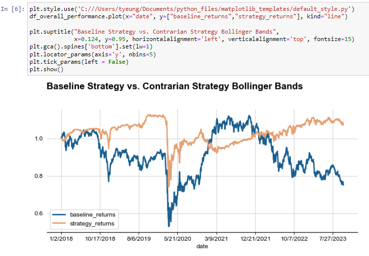
And if shorting is not allowed…

In both cases, we see the strategy outperforming as expected. If a momentum-seeking strategy gives us negative returns, then taking the negative of that strategy will do the opposite.

So… can we do even better?

4. Fundamental + Technical Strategies

It turns out that adding specialized financial knowledge does help technical analysis strategies do better. We know, for instance, that utility and consumer staple firms (mentioned above) often revert to a mean. Earnings at these firms tend to gravitate to a certain level, which constrains how far their share values can move. Most water utilities even have their return on equity (ROE) capped by regulators to ensure they don’t overcharge customers!

Let’s re-run the contrarian strategy on these types of firms. Here, I use Thomson Reuters standards to select only companies categorized as “consumer non-cyclicals” and “utilities.”

funda_file = "fundamental_data.csv" # adding fundamental data file
df_funda = pd.read_csv(funda_file)

tickers = [] # keep same format as above
df_columns = list(df_input)

for ticker in df_columns:
    try:
        trbc = df_funda.loc[df_funda['RIC'] == ticker, 'trbc_sector_name'].iloc[0]
        if trbc in ("Consumer Non-Cyclicals", "Utilities"):
            tickers.append(ticker)
    except: pass

Then run the graphing code to get our output…

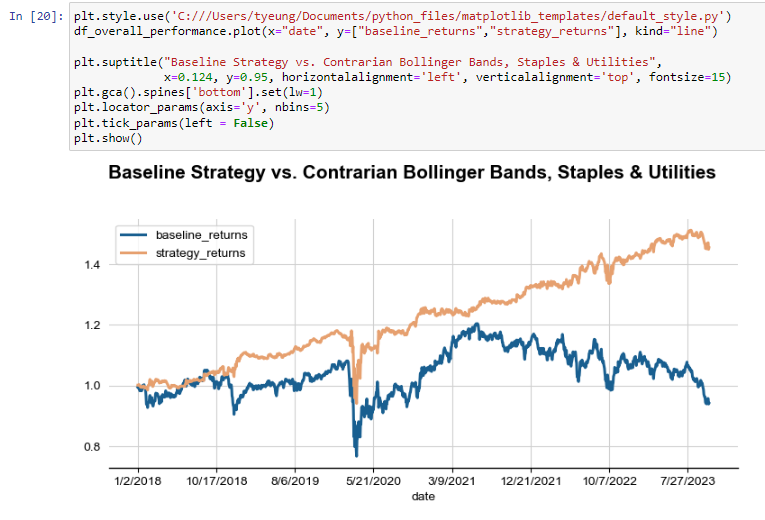
And we see our performance surge! In this case, our contrarian Bollinger Bands help us outperform all staples and utilities stocks by 51.4% over roughly five years — a stunning 7.8% annualized rate of return.

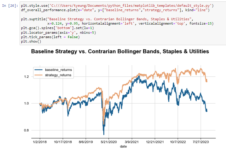
Even if we disallow short positions, our performance is still remarkable.

Let’s then consider the alternative — using momentum-seeking strategies to help us choose riskier stocks.

Here, we’ll take all companies with an Altman Z-score of less than 1.2 — a quantitative sign of weak financial health. All else equal, we would expect this group of stocks to underperform over the longer run. Can our Bollinger Band strategy defend us against losses?

for ticker in df_columns:
    try:
        z_score = df_funda.loc[df_funda['RIC'] == ticker, 'z_score'].iloc[0]
        if z_score < 1.2:
            tickers.append(ticker)
    except: pass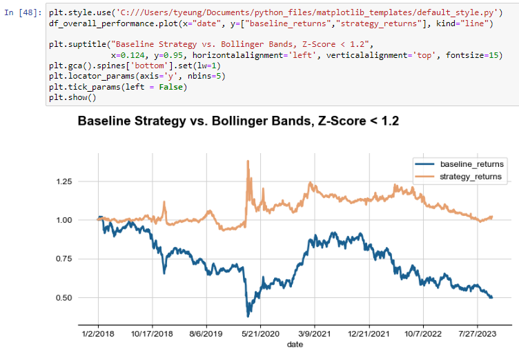

Indeed, it does! Here, we see the Bollinger Band strategy indeed doing well against failing firms, especially during the initial years. (The performance gets even better if we refresh numbers and rebalance our portfolio). That’s because falling stocks are sold before they can do too much damage.

In other words, knowing when to use technical analysis strategies involves understanding fundamental analysis as well as technical strategies.

Bollinger Bands: Further Tests

Of course, we can continue to try more tests. Let’s explore the double bottom strategy. This tactic buys stocks the second time they cross under the lower Bollinger Band and sells them once they cross above the higher band.

And here’s that strategy in algorithmic form. This code fits into the same for loop as before and replaces our "df["position"] = (df.bb_bbhi - df.bb_bbli).astype(float)" line with a slightly more complex piece of logic:

    df["bb_bbli_prev_day"] = df["bb_bbli"].shift(periods=1) # for comparing 2 days
    df["position"] = 0  # create starting positions of all zeros
    bbli_streak = 0 # create starting streak of zero
    
    for index, row in df.iterrows():

        # add to the streak counter if needed. Consecutive days not counted
        if (row["bb_bbli"]) == 1 and (row["bb_bbli_prev_day"]) == 0:
            bbli_streak += 1 
            
        # if streak >= 2, add buy signal
        if bbli_streak >= 2:
            df.at[index, "position"] = 1
        
        # if hit a high band, default to a zero position and reset streak
        if row["bb_bbhi"] == 1:
            bbli_streak = 0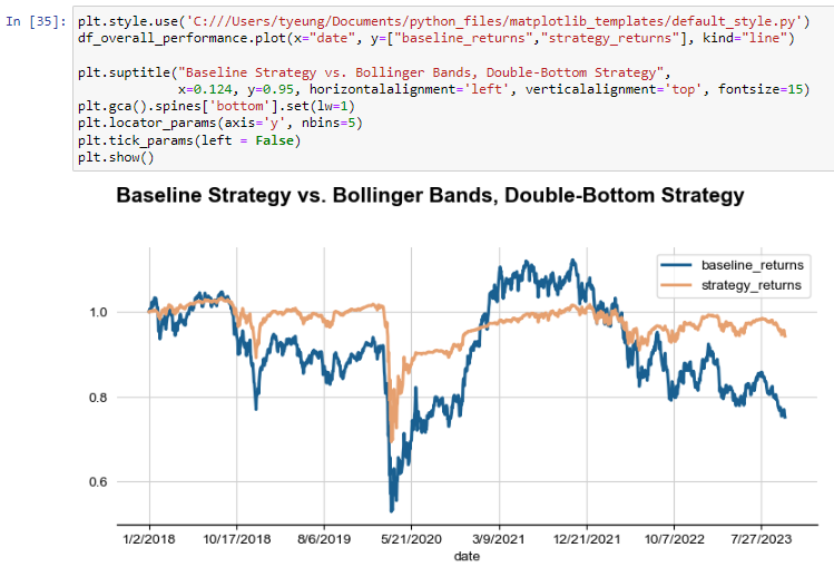

We can also add the two bolded lines of code to make the system sell short the stock once we hit the upper band.

        # if hit a high band, sell position and reset streak
        if row["bb_bbhi"] == 1:
            df.at[index, "position"] = -1
            bbli_streak = 0
    
    df["position"].replace(0, method='ffill', inplace=True)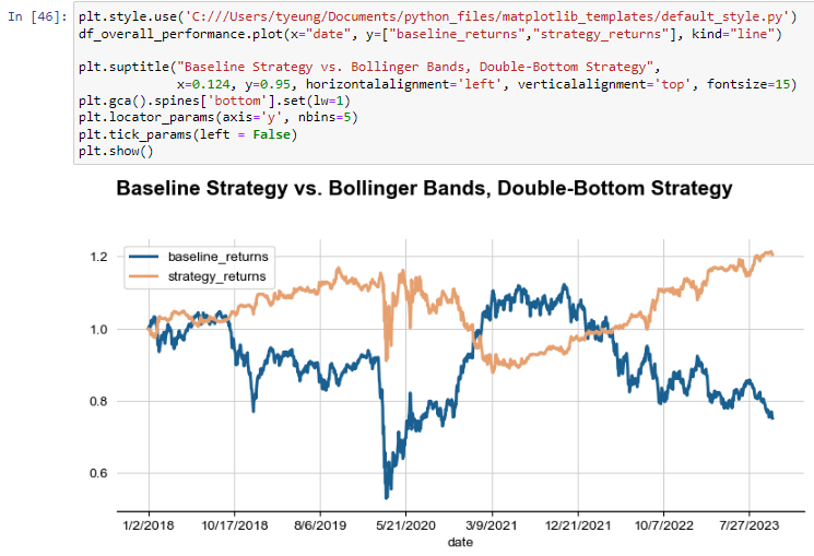

However, we eventually see that Bollinger Bands without fundamental data is much like peanut butter without jelly. Or a road trip without $100 worth of snacks on board.

It doesn’t work as well.

Even that final test of a double bottom strategy had months where the portfolio underperformed. And in the end, its 45% outperformance still lags the 50%-plus returns we saw with fundamental/technical hybrid models.

That’s why I highly recommend you read through my work on MarketMasterAI, a stock-picking AI algorithm that combines fundamental and technical data into a low-turnover trading strategy. It’s a system that uses hundreds of parameters and millions of datapoints to sense patterns like the ones found here… and all with greater backtesting and validation rigor.

Final Thoughts on Bollinger Bands

Bollinger Bands are a Rorschach test for investors. Some will see the stocks hit the bottom Bollinger line and think, “It’s time to buy.” These contrarian thinkers often become value investors — buying the dips and selling on peaks.

Meanwhile, other investors will see stocks hit the upper Bollinger band and get excited about buying. These trend-following investors tend to favor growth companies that can keep going up over time.

Our study here shows that both sides could be right… provided they use the right strategy for the class of stocks they buy. Stable companies need a mean-reverting strategy, while riskier ones should use a breakout one. You need the right tool for the job.

That’s why investors need to use technical analysis as a way to enhance their fundamental knowledge about a company… not supplant it entirely. Although no billionaire investor has ever made their fortunes solely from reading stock charts, you can be sure that the top traders have used price movements plenty to help give themselves an edge.

To learn more about gaining these advantages, click here to read about MarketMasterAI, my quantitative stock-picking strategy. The machine-learning system is 100% free (for now) and combines much of what we’ve talked about here into a robust trading system that has provenly outperformed the markets.

On the date of publication, Tom Yeung did not hold (either directly or indirectly) any positions in the securities mentioned in this article. The opinions expressed in this article are those of the writer, subject to the InvestorPlace.com Publishing Guidelines.